The women participation in economic activities in today world increase that affect the equality in gender. However, some critics believe that women still be treated unequally to men and may get fewer benefits in the same efforts. Therefore, this essay will examine the assumption that women may earn less income than men regarding the income in the case of Australia in three steps. First, this essay will discuss the relating current discourses on gender income inequality and its current concepts that explain factors that influence women`s income. Second, using several multiple regression models, this study will examine the main factors of women income. Third, this essay expands the position of satisfaction as the determining factor in gender discourse. The main findings of this study are the gap income relating gender still become an essential issue where education years is the most significantly dominant factor of the income. Moreover, the study examined that the average of income women significantly under national minimum wages of Australia and the effect on job satisfaction is considered to be an active factor in variable income.
Income and Women
The women participation in the workforce may be an increase in the modern world yet dynamics in recent decades. World Bank explained that the participation of women of 15 to 64 years old slightly decreases from 51.37% to 48.8 % (Figure 1). However, Australia has a significant increase from 52.2% in 1990 to 59.21% in 2014 which means almost six from ten women in the age 15 to 64 are workers (ILO, 2018). Therefore, It may be questioned that the reason and factors that Australia has a different direction from the world.
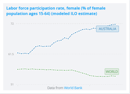
Figure 1. Labour force participation rate of women in Australia and the World
However, the obstacle relating to the income may still occur in all of the countries. World Economic Forum (WEF) made an index to measure the wide of the gap the world. In 2017, global gap index is 0.68 which means that the average gap between man and women is 32% (WEF, 2017, p. 8). In details, New Zealand as a country that has similar characteristics with Australia is the best eight which has the gap rate almost 0.8 while Australia has gap rate 0.731 in the rank of 35 WEF (2017, p. 8). Therefore, although it still has a gap, Australia is better than the majority of world countries.
Also, the high rate of women participation in Australia is not directly to be the conclusion that Australia`s women worker has no crucial issues. This income gap is still something that the government needs to be solved. Stewart, Voitchovsky and Wilkins, (2017, p. 258) demonstrated that in the highest 10% of workers in Australia only one-fourth that it comes from women. It might reflect that Australian women worker difficult continuously increase his career as well as a salary to the top.
[AdSense-A]
What Affect Income?
Constructing determinant factor of income may be broad and complex that may be caused some cases where discrimination become the cause (Kobe University, 2016, p. 20). However, the study will construct mainly the factors by three characteristics which are education level, marital status, and working hours.
First, education level may become and dominant factor to increase the wage. Wolla and Sullivan (2017, p. 2) explain that relationship between education and income is stable because of the philosophy of education as an ‘investment of human capital’. He said that one of the main reasons people have to work in line with the term ‘investment of human capital’ is an approach to have a good job that may be measured with the well-paid.
Second, many types of research are conducted to analyse the relationship between working hours and income. Both traditional and modern wage models made to equal with working hours. Moreover, the wages model set minimum wages and overtime fees that affect the increase in income (TFT, 2016, p. 2). However, Giannis (2014, p. 16) found with the model of wage with a relative wage that income and working hours have a negative relationship. Therefore, this study considers to include working hours to find the situation of working hours in women workers in Australia.
Third, Bracher (1990, p. 138) studied that in Australia that income and first marriage rates have a significant negative relationship. It means that married women may earn an income less than those who still single. The reduce the income of married women is caused by the productivity of married women may less than single women. This is because, in the example of America society, they spend much time than the man on activities beyond main working (BLS, 2015); for instance, women have to spend much time to their children, kitchen and food activities, manage and purchase for necessities, and sometimes laundry and cleaning activities.
Data and Methodology
Data and Variables
The study uses The Australian Survey of Social Attitudes (AuSSA) 2012 which is conducted by Australian Data Archive (ADA) under International Social Survey Project (ISSP). The survey aims to chart Australian opinions about their lives with 1620 samples and 217 variables (ADA, 2015, pp. 1–7). However, this essay will use several variables that related to income equality in the survey.
The study will analyse one dependent variable that is gross monthly income of Australia. The variable is collected in Australian dollars with the full range with the lowest is $10 to the highest $ 1 million. In one case, the income data will be transformed to ordinal data of low, middle, and high category in order to find the causality with the satisfaction variable. The main struggling issue in this variable is many outliers; for instance, the median data of variable is $4,400 which reflects that the majority of data are summed to under $ 5,000 even though the maximum data is $ 1 million. The outliers in income may be caused by the small number or high earn wages of few people that not equal with the majority of the rest of Australian income.
On the other hand, the study assigns four independent variables which are work hours, the education years, marital status, and satisfaction. The education years and working hours are on the ratio scale, while gender, marital status, and satisfaction scale are in nominal and ordinal scale. In details, the ‘working hours’ refers to how long the worker spend their time to work in a week including overtime where Australian spend their time on average at 37.92 hours weekly or 7.5 hours per day in five days’ work. The education years refers how long the workers took their last education. It helps to identify the effect of educational experience to determine the income. Marital status simply classified as married and not married. In order to make it clearer, the terms that classified in divorce and civil partnership will be excluded as marriage. Satisfaction variable is an ordinal scale data that explain the range of satisfaction that the worker feels in the range of dissatisfied to satisfied. In some cases, the satisfaction data will reform to the most straightforward category of dissatisfied, neither satisfied nor dissatisfied, and satisfied.
Methodology
This study uses three statistical approaches to answer the research problem. First, in order to find the position of average women wage with the national minimum wages, the analysis need t-test with the alternative hypothesis is Australian women worker earn income on average less than minimum wages of Australia.
On the other hand, the essay constructs five models of multiple regression to make a test some variable on different treatments. Models will use dependent and independent variables that be formed to some dummy variables.
The final statistical methods that being adopted in this study is the chi-square test in order to find the relation between satisfaction and the income. Although income variable is in the form of ratio scale, the variable will be transformed to categorical data with three classes of income which are low, middle, and high. These categorical class are determined with the boundaries of three quartiles.
Result
The study among workers in AuSSA 2012 descriptively shows that male has a higher income than female. According to Figure 2, the median of the male is $ 5,500 while women are 3,600 that means the difference between male-female is $1.900 or 52% higher of female income. However, the main obstacle of this data is several outliers that reflects some people of this survey were very rich that makes the distribution is unable to chart deeply.
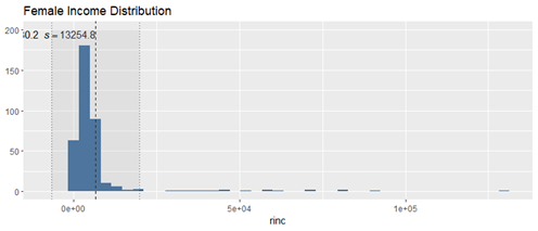
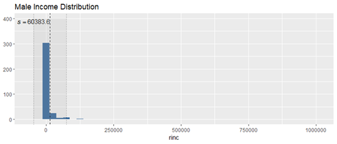
Figure 2. Income Distributions on Gender
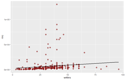
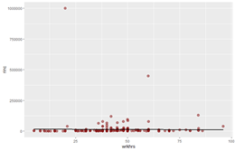
Also, we cannot say the inequality of gender yet in Australia because the survey shows that on average male spend 32.8 % much time rather than female. Figure 3 shows Australian male tends to spend their time to work close to a normal distribution which means the average is equal to the median at 42 hours weekly, while women workings hours average is less from the median. Therefore. It has descriptively explained from figure 3 that female quantitatively less productive than male om regarding working hours.
Income vs Work Hours (Female) Income vs Work Hours (Male)
Income vs Education Years (Female) Income vs Education Years (Male)
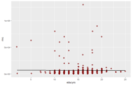
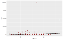
Figure 3. Scatter Plot Income, Education Years, and Work Hours on Gender
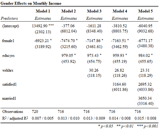
In details, male earn average $ 10.733.57 monthly whereas female only $ 5.522,57 monthly on average. It means that the gap income of Australia regarding gender almost 100%. It is supported with the set of the regression model in Table 1 that shows the significant negative effect (α=.05) in almost all models which mean women have less salary than men in between $6.000-$7.000. Moreover, Education years also has significantly positively affected (α=.05) to income all models of multiple regression in Table 1 which reflects educational experience may be considered as a factor to increase the income. Therefore, it is clear that that income was constructed by the influence significantly the gender and education years while satisfying the job and marital status has a less significant effect.
Table 1. Multiple Regression Model Tabulation
On the other hand, discourse of gender equality related to the sufficiency income especially female in Australia. According to Fair Work Australia (2008, p. 1), the national minimum wages of Australia is $18.93 per hours or $3.028 per month with the assumption that workers have to work eight hours per day in twenty days per month. There the study has tested both male and female on their income where the null hypothesis is the Australian on average in a particular gender have an income of more than $3028 or more. The result of the test is both male and female successfully rejected hypothesis null at significant level .01 which means the average test of Australian`s income based on gender less than national minimum wages. However, we cannot declare that the majority of Australian has income less than minimum wages because the data distribution is slightly wide; for instance, the standard deviation of the female is $12,907 while the male is $60.292.
Table 2. Satisfaction on working women
crosstab.
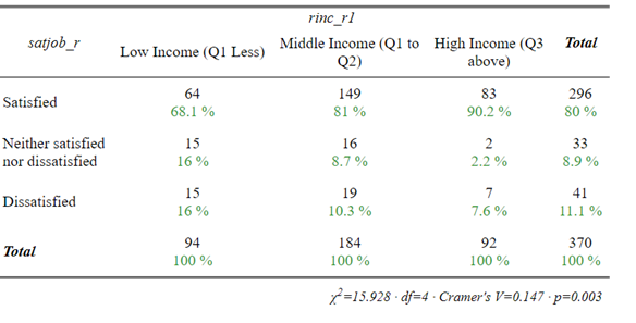
However, the insignificant effect of satisfaction on income brings the test to another context. Table 2 shows crosstab as a result of filtered women data on satisfaction on their job related to the classification of three classes of income based on quartiles. The lowest level is all income that in the amount between zero to the first quartile, middle income is all amount income between second to the third quartile, and the highest income level is all income above the third quartile. The table shows that the more prominent worker`s salary, the more satisfied worker will feel. The chi-square test of the data resulted that the in the level significant of 0.01 the satisfaction of a job that has related with the income. This result may complete the regression multiple in model four and five (Table 1) that no affect satisfaction to salary (income become independent). On the contrary, income that affect satisfaction (Table 2).
Therefore, Australia`s women participation in workforce increase steadily. However, an issue of income inequality regarding gender in Australia often is debated in the last years. This study has answered descriptively that Australian women earn money less than men in line with women quantitatively spend their time working less as well. Regression models show that education years strongly affect the level of income yet working hours, satisfaction, and marital status failed to prove as important factors. Furthermore, the income of women on average significantly less than minimum wages of Australia. This study also replaced and justified satisfaction as not an influencing factor to women income, but an influenced factor to the income. Therefore, it is clear that the discourse of gender inequality regarding income still needs to be propagated, especially factors that invisible in this study, for instance, sociological factors.
References:
ADA (2015) ‘Australian Survey of Social Attitudes, 2012’.
BLS (2015) American Time Use Survey. Available at: https://www.bls.gov/tus/charts/household.htm (Accessed: 15 November 2018).
Bracher, M. (1990) EXPLAINING FIRST MARRIAGE TRENDS IN AUSTRALIA, Source: Journal of the Australian Population Association. Available at: https://www.jstor.org/stable/pdf/41110589.pdf?refreqid=excelsior%3A1b7adadd347c09b289c3ffc88b7c0d30 (Accessed: 13 November 2018).
Fair Work Australia (2008) Minimum Wages. doi: 10.7551/mitpress/9780262141024.001.0001.
Giannis, M. (2014) ‘The Effect of Relative Wage on Hours Worked’, Honors Projects. Available at: https://digitalcommons.iwu.edu/cgi/viewcontent.cgi?article=1127&context=econ_honproj (Accessed: 15 November 2018).
ILO (2018) Labor force participation rate, female (% of female population ages 15-64) (modeled ILO estimate) | Data, ILOSTAT Database. Available at: https://data.worldbank.org/indicator/SL.TLF.ACTI.FE.ZS (Accessed: 15 November 2018).
Kobe University (2016) Examining the Factors Affecting Personal Income: An Empirical Study Based on Survey Data in Chinese Cities. Kobe. Available at: http://www.econ.kobe-u.ac.jp/activity/graduate/pdf/王李蕙.pdf (Accessed: 15 November 2018).
Stewart, M., Voitchovsky, S. and Wilkins, R. (2017) Women and top incomes in Australia. ANU Press. Available at: https://www.jstor.org/stable/pdf/j.ctt1zgwj9q.17.pdf?refreqid=excelsior%3A507d5014bbf4834fe83c8d18efd19bcd (Accessed: 13 November 2018).
TFT (2016) Wages and Working Hours. Available at: http://www.oxforddictionaries.com (Accessed: 15 November 2018).
WEF (2017) The Global Gender Gap Report 2017 Insight Report. Available at: http://www3.weforum.org/docs/WEF_GGGR_2017.pdf (Accessed: 15 November 2018).
Wolla, S. A. and Sullivan, J. (2017) Education, Income, and Wealth. Available at: https://fred.stlouisfed.org/graph/?g=7yKu. (Accessed: 15 November 2018).
Appendix 1. R Output
income <- readRDS(“aussa2012.rds”)
Cleaning Process
#Remove NA Data
income2 <- income %>% select(work,rinc,sex, educyrs, wrkhrs, marital, satjob)
income2 <- income2 %>%
mutate(mark = 0)
income2 <- income2 %>%
mutate(mark = replace(mark, complete.cases(income2), 1))
income2 <- income2 %>%
filter(mark == 1)
frq(sex)
#remove unemployment
income2 <- rec(income2, work, rec = “1=1;2:3=0”, append = TRUE)
income2 <- income2[income2$work_r==1,]
#remove zero income
income2 <- rec(income2, rinc, rec = “0=0;1:1000000=1”, append = TRUE)
income2 <- income2[income2$rinc_r==1,]
Creating Dummy Variables
#sex
income2 <- rec(income2, sex, rec = “1=0;2=1”, append = TRUE)
income2 <- var_rename(income2, sex_r = female)
income2$female <- set_label(income2$female, label = “Gender”)
income2$female <- set_labels(income2$female, labels = c(“Male” = 0, “Female” = 1))
income2$female <- to_factor(income2$female)
income2$male <- ref_lvl(income2$female, lvl = 1)
#marital
income2 <- rec(income2, marital, rec = “1=1;2:6=0”, append = TRUE)
income2 <- var_rename(income2, marital_r = married)
income2$married <- set_label(income2$married, label = “Married Status”)
income2$married <- set_labels(income2$married, labels = c(“Married” = 1, “Not Married” = 0))
income2$married <- to_factor(income2$married)
income2$Unmaried <- ref_lvl(income2$married, lvl = 1)
#satisfied
income2 <- rec(income2, satjob, rec = “1:3=1;4:7=0”, append = TRUE)
income2 <- var_rename(income2, satjob_r = satisfied)
income2$satisfied<- set_label(income2$satisfied, label = “Satisfied”)
income2$satisfied <- set_labels(income2$satisfied, labels = c(“Satisfied” = 1, “Not Satisfied” = 0))
income2$satisfied <- to_factor(income2$satisfied)
income2$notsatisfied <- ref_lvl(income2$satisfied, lvl = 1)
Regression Model
#Regression
model.1 <- lm(rinc ~ female, data = income2)
model.2 <- lm(rinc ~ female+educyrs, data = income2)
model.3 <- lm(rinc ~ female+educyrs+wrkhrs, data = income2)
model.4 <- lm(rinc ~ female+educyrs+wrkhrs+satisfied, data = income2)
model.5 <- lm(rinc ~ female+educyrs+wrkhrs+satisfied+married, data = income2)
tab_model(model.1, model.2, model.3, model.4, model.5, digits = 2, pred.labels = c(“Intercept”, “Female”, “Education Years”, “Education Degree”, “Married”, “Not Married (ref. = incl. civil partnership and divorce)”, “Happy with Their Life”,”Not Happy with Their Life”),
dv.labels = c(“Model 1”, “Model 2”, “Model 3”, “Model 4”, “Model 5”), title = “Gender Effects on Monthly Income”, show.se = TRUE, show.ci = FALSE, collapse.se = TRUE, p.style = “asterisk”)
T-test
female.income <-income2[income2$sex==2,]
male.income <-income2[income2$sex==1,]
t.test (female.income$rinc, mu=3028)
t.test (male.income$rinc, mu=3028)
sjp.frq(male.income$rinc, type = “hist”, title = “Male Income Distribution”, show.mean = TRUE)
sjp.frq(female.income$rinc, type = “hist”, title = “Female Income Distribution”, show.mean = TRUE)
plot_scatter(female.income, wrkhrs,rinc, colors = “#8B1A1A88”, dot.size = 3, fit.line = “lm”)
plot_scatter(male.income, wrkhrs, rinc, colors = “#8B1A1A88”, dot.size = 3, fit.line = “lm”)
plot_scatter(female.income, educyrs, rinc,colors = “#8B1A1A88”, dot.size = 3, fit.line = “lm”)
plot_scatter(male.income, educyrs, rinc, colors = “#8B1A1A88”, dot.size = 3, fit.line = “lm”)
Chi Square Test
income2 <- rec(income2, satjob, rec = “1:3=1;4=2;5:7=3”, append = TRUE)
income2$satjob_r<- set_labels(income2$satjob_r, labels = c(“Satisfied” = 1, “Neither satisfied nor dissatisfied” = 2, “Dissatisfied”=3))
income2$sex<- set_labels(income2$sex, labels = c(“male” = 1, “female” = 2))
sjt.xtab(income2$satjob_r, income2$sex, show.col.prc = TRUE)
sjt.xtab(male.income$satjob_r, male.income$rinc, show.col.prc = TRUE)
#ChiSquareTest #female
female.income <- rec(female.income, rinc, rec = “1:2000=1;2001:5462=2;5463:130000=3”, append = TRUE)
female.income$rinc_r1<- set_labels(female.income$rinc_r1, labels = c(“Low Income (Q1 Less)” = 1, “Middle Income (Q1 to Q2)” = 2, “High Income (Q3 above)” = 3))
female.income <- rec(female.income, satjob, rec = “1:3=1;4=2;5:7=3”, append = TRUE)
female.income$satjob_r <- set_labels(female.income$satjob_r, labels = c(“Satisfied” = 1, “Neither satisfied nor dissatisfied” = 2, “Dissatisfied”=3))
sjt.xtab(female.income$satjob_r, female.income$rinc_r1, show.col.prc = TRUE)
frq(female.income$rinc_r1)


Leave a Reply